Week 3, skill booster 2
Finding what stands out.
Blob detection with OpenCV, taken all the way: SimpleBlobDetector, Laplacian and Difference of Gaussians and Determinant of Hessian written from scratch, a classical detector for cones, cubes and rings, and a YOLOv8 study that finds the dataset's test split leaks. Every number below is measured against ground truth.
- dots
- 0.998 F1 on the three photos (217 hand checked dots), 0.02 px median center error on synthetic truth
- pieces
- 6 of 6 pieces found and classified, mean mask IoU 0.942 against SAM annotations
- yolo
- mAP50 0.588 to 0.820 on held out clips, ball AP50 0.00 to 0.57
- stack
- Python, OpenCV, NumPy, Ultralytics, C++17
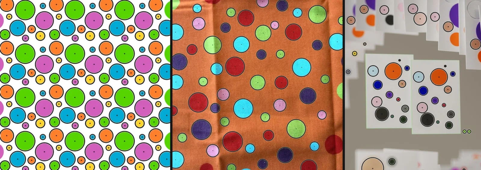
Two options, two challenges. All of it.
The Week 3 skill booster is object detection: OpenCV blob detection or training a YOLOv8 model. Here is each task as given, and what the repo ships for it.
-
Option 1
OpenCV blob detection
Use SimpleBlobDetector to detect the polka dots in the three images. Try to filter blobs by size or color.
- Hand checked ground truth for every dot in all three photos, so detectors are scored, not eyeballed.
- SimpleBlobDetector three ways: on grayscale, per learned palette color, and on a background contrast map. Filters by radius, color name, circularity, convexity and inertia.
- Sub pixel edge fit for every dot, which also rejects squares, stars and gaps between dots.
-
Challenge 1
LoG, DoG, DoH, contours
Detect objects using other methods.
- Scale space detectors from scratch in CIELAB, with an image pyramid, a streamed search and SIFT style sub pixel refinement. Checked against scikit-image.
- Contour filtering on color edges.
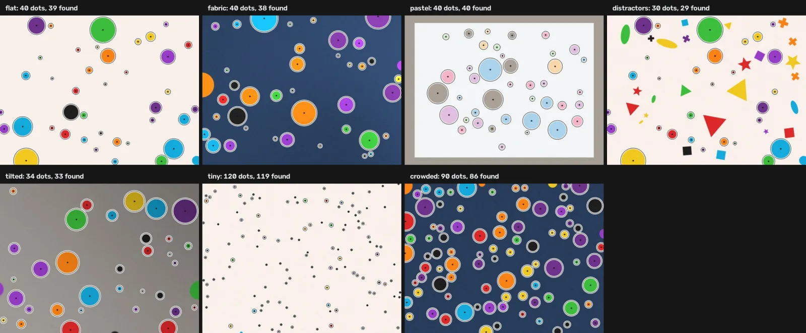
- A synthetic benchmark with exact truth: fabric, pastels, distractor shapes, perspective, tiny and crowded dots.
-
Challenge 2
Cones, cubes and rings
Detect and classify the cones, cubes and rings in the objects file, with accurate contours or bounding boxes.
- Classical, no training: saturation seeds, hue clustering, hysteresis growth, a convexity defect cut between touching cubes.
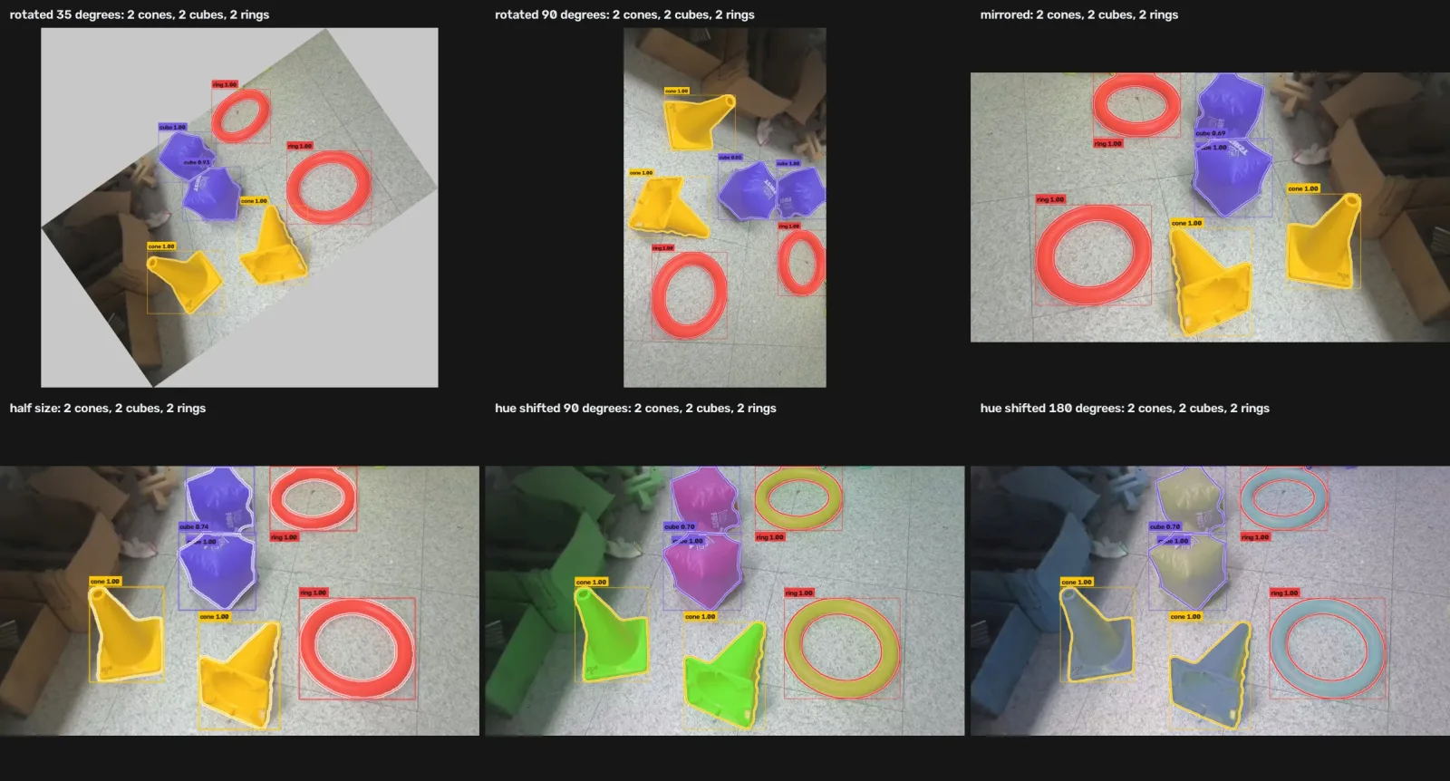
- Classified by geometry, not color: holes, convexity and triangularity. Survives rotation, mirroring, scaling and hue shifts.
- Scored against SAM 2 masks, the annotation trick from the lecture.
-
Option 2
YOLOv8
Train your own YOLOv8 model, explore Roboflow's preprocessing and augmentation, and see if you can improve performance.
- The notebook's football dataset without a Roboflow key, and a leak in its split: every test clip also appears in training.
- Roboflow's tile preprocessing and augmentation catalogue, reimplemented with boxes that follow the pixels.
- Sliced inference for the 11 pixel ball, and one COCO style scorer for every experiment.
Seven detectors, three photos.
Every detection below is precomputed by python -m week03 docs and scored against the hand checked annotations. Rings are found dots, red rings are false positives and dashed circles are dots the method missed. Hover or tap a dot for its measurements.
Dots cut in half by the frame are optional, and on the third photo the out of focus cards behind are not scored either way.
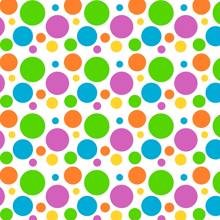
found false positive missed not scored
Laplacian of Gaussian
- F1
- 0
- Precision
- 0
- Recall
- 0
- Time
- 0
Dots by color
How a blob detector sees.
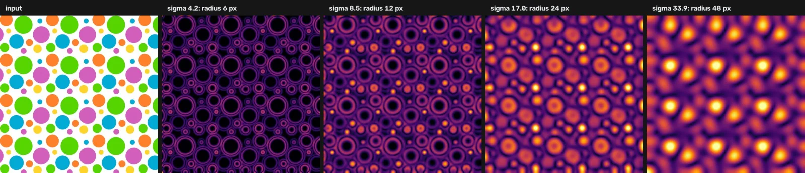
A dot of radius r answers loudest to a Laplacian of Gaussian of width r divided by the square root of two. Sweep the width and every dot lights up at its own scale, so one search finds both where each dot is and how big.
Run on CIELAB instead of gray, the response is measured in Delta E, the unit of visible color difference. A cyan dot on orange fabric has almost the same brightness as the cloth; in color it is obvious.
From candidate to measured dot
-
Detect
3x3x3 maxima of the response stack, searched on the color magnitude and on each signed channel, three scale slices at a time.
blobs.detect_scale_space -
Refine
A quadratic fit through the 27 neighbors moves each peak to sub pixel position and fractional scale, as SIFT does.
offset = -H⁻¹ g -
Drop sidelobes
A disk's Laplacian is ringed by weaker, opposite sign response. A peak that is the negative of a much stronger neighbor is its echo.
cosine < -0.7 -
Fit the edge
Along 48 rays, find where the color crosses halfway from dot to background. A robust circle, then an ellipse, fits those points.
Kasa fit + cv2.fitEllipse -
Verify
Uniform inside, a different color just outside, and a surround that is itself one color. That rejects squares, stars and gaps.
fill, leak, surround -
Filter
By radius, by color name, by contrast, by roundness. The same knobs SimpleBlobDetector has, measured after the fit.
--colors red --min-radius 10
Two bugs the benchmark caught.
Both looked fine on the photos and were only visible against exact truth.
Every method was 0.53 px off. Identical error for seven different detectors meant the truth was wrong, not the detectors. The scene renderer drew dots on a 4x supersampled canvas without the half pixel shift between grids. After the fix, clean dots are located to 0.02 px.
Pale pink dots vanished. Suppressing sidelobes by distance and strength alone deleted faint dots beside black ones. A sidelobe is its parent's response with the sign flipped in the same channels; pink next to black lives mostly in the a channel, which black cannot produce. Checking direction, not just size, brought them back.
Benchmark
F1 on the three photos, then on 21 synthetic scenes where the true center and radius of every dot is known. Generated by python -m week03 benchmark.
| Detector | Flat print136 dots | Fabric53 dots | Cards28 dots | Synthetic F1 | Center error | Radius error |
|---|---|---|---|---|---|---|
| SimpleBlobDetector, grayscale | 0.903 | 0.000 | 0.923 | 0.883 | 0.02 px | 1.0% |
| SimpleBlobDetector, per palette color | 0.989 | 0.809 | 0.667 | 0.916 | 0.02 px | 0.9% |
| SimpleBlobDetector, background contrast | 0.981 | 0.971 | 0.982 | 0.984 | 0.02 px | 1.0% |
| Contours on color edges | 0.989 | 0.918 | 0.923 | 0.963 | 0.02 px | 0.9% |
| Laplacian of Gaussian | 1.000 | 0.981 | 1.000 | 0.998 | 0.02 px | 1.0% |
| Difference of Gaussians | 1.000 | 0.991 | 1.000 | 0.997 | 0.02 px | 0.9% |
| Determinant of Hessian | 1.000 | 0.971 | 0.982 | 0.998 | 0.02 px | 0.9% |
- SimpleBlobDetector
- On grayscale it cannot see a dot as bright as its background: zero of 53 on the fabric. Given a color contrast map it gets 0.979.
- Scale space
- LoG, DoG and DoH agree within a dot or two everywhere. DoH is near zero on straight edges, which helps next to card borders.
- Errors
- Median over matched dots on synthetic scenes. The photo annotations come from the same edge fit, so only precision and recall are scored there.
Cones, cubes and rings, without a neural network.
No training data, so the detector has to reason. Game pieces are saturated plastic on gray tile, the pieces touch, and the shaded side of a cube is barely colored at all.
Drag to compare with the SAM masks.
All 6 pieces found and labeled with no false positives: mean mask IoU 0.942 and box IoU 0.955 against masks from SAM 2, prompted with hand drawn boxes and checked by eye. Refining the outlines with GrabCut was tried and scored 0.932, so it stays off.
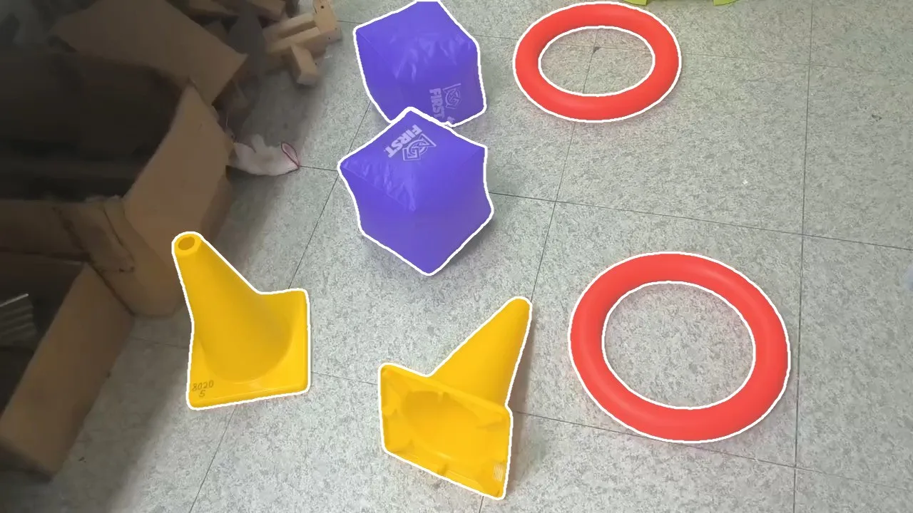
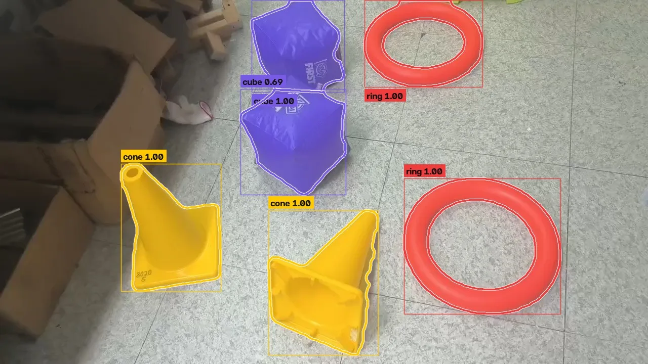 SAM 2 truth
Classical detector
SAM 2 truth
Classical detector
Geometry decides the class
- RingA large hole near the middle.
- CubeA convex polyhedron has a convex silhouette: solidity near 1.
- ConeConcave where the body meets the base flange, and a convex hull close to a triangle, standing or lying down.
Touching cubes: two thick centers in the distance transform, two notches where the silhouettes meet. The cut runs between the notches. A single cone has one thick center, so it is never cut.
| Piece | Solidity | Hole | Triangularity | Mask IoU |
|---|---|---|---|---|
| cone | 0.86 | 0.00 | 0.73 | 0.969 |
| cone | 0.87 | 0.00 | 0.83 | 0.932 |
| cube | 0.94 | 0.00 | 0.61 | 0.925 |
| cube | 0.96 | 0.00 | 0.70 | 0.911 |
| ring | 0.99 | 0.37 | 0.62 | 0.974 |
| ring | 0.99 | 0.45 | 0.61 | 0.938 |
Rotate it, mirror it, recolor it.
Nothing in the classifier knows that cones are yellow or where the camera is. The same image rotated, mirrored, halved and hue shifted until the cones turn blue still reads 2 cones, 2 cubes, 2 rings in all 6 versions.
Bonus: the shapes file.
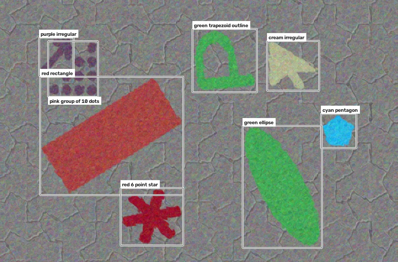
The Week 3 folder also had painted targets. Segmented by Delta E from the local background, then classified with the Week 2 SUAS template matcher plus ellipses, n pointed stars and dot groups.
YOLOv8, and a leak in the data.
The notebook trains on Roboflow's football players dataset: 372 broadcast frames at 1920x1080 with players, goalkeepers, referees and the ball. File names start with a clip id, and the random split puts frames of every test clip into training too, often a second apart.
So every model is scored twice here: on Roboflow's split, and on a clean split that holds out whole clips.
| Experiment | Test split | Inference | mAP50 | mAP50-95 | Ball | Goalkeeper | Player | Referee |
|---|---|---|---|---|---|---|---|---|
notebook-split | Roboflow (leaky) | whole frame, 640 px | 0.609 | 0.395 | 0.000 | 0.844 | 0.965 | 0.628 |
baseline | held out clips | whole frame, 640 px | 0.588 | 0.382 | 0.000 | 0.861 | 0.962 | 0.530 |
offline-aug | held out clips | whole frame, 640 px | 0.580 | 0.347 | 0.000 | 0.776 | 0.944 | 0.599 |
hires-inference | held out clips | whole frame, 1280 px | 0.419 | 0.268 | 0.000 | 0.142 | 0.943 | 0.590 |
tiles | held out clips | whole frame, 640 px | 0.380 | 0.215 | 0.100 | 0.216 | 0.896 | 0.308 |
tiles | held out clips | sliced, 640 px | 0.820 | 0.567 | 0.569 | 0.945 | 0.965 | 0.799 |
On their own test sets the same recipe scores 0.609 mAP50 on Roboflow's split and 0.588 on held out clips. Those are different frames, so the gap mixes the leak with how hard each test set is.
A controlled check scores both models on the same 11 frames: Roboflow test frames from the two held out clips, whose neighboring frames the leaky model trained on and the clean model never saw. The leaky model scores 0.712 mAP50 and the clean one 0.660 (+0.052); on referees, the class that depends most on context, 0.868 against 0.675. 11 frames is a small sample, and the leaky model also had more training frames (298 against 259), but both comparisons point the same way. Every row below the first uses held out clips.
The baseline finds players well but the ball not at all: ball AP50 0.000, because an 11 px ball is under 4 px after resizing to 640.
Training at 1280 px does not fit an 8 GB M1 (over 25 minutes per epoch, swapping). Running the baseline weights at 1280 px instead gives mAP50 0.419 (ball 0.000, goalkeeper 0.142): every object is suddenly twice the size the model learned. Resolution has to change in training and inference together, which is what tiling does.
Roboflow style offline augmentation (two extra copies, the same number of training steps) gives 0.580 mAP50. Ultralytics already augments online with mosaic, HSV jitter, flips and scaling, so the extra copies mostly repeat what it does.
tiles: trained on 960x540 tiles, then run on overlapping tiles plus the whole frame and merged. mAP50 0.820 and ball AP50 0.569, against 0.380 and 0.100 for the same weights on whole frames.
Drag to slice.
The same model on a held out frame: whole frame at 640 px on the left, sliced into overlapping 960x540 tiles plus the whole frame on the right.
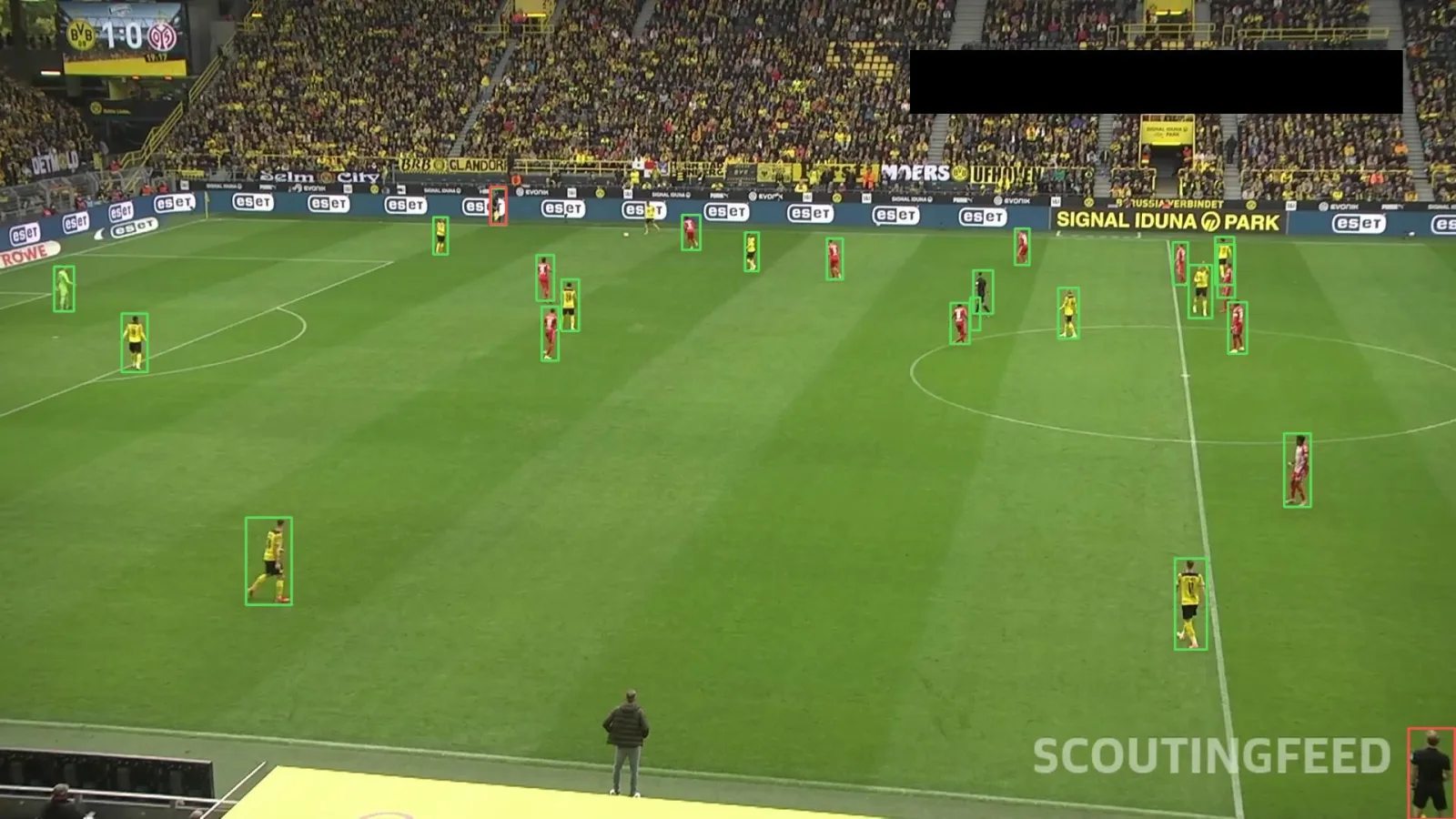
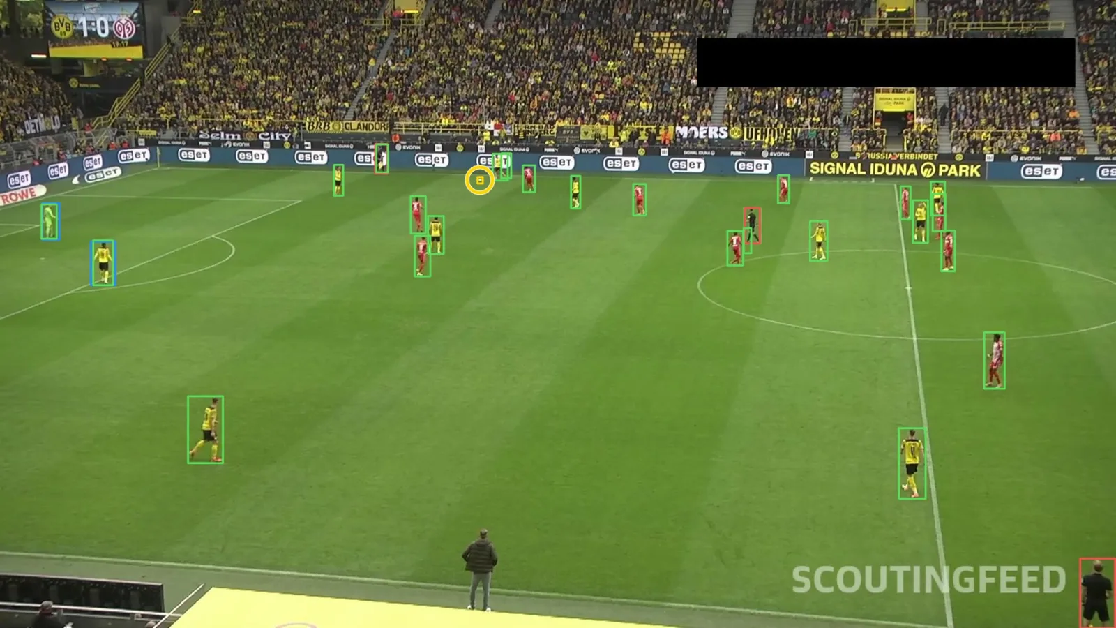 Whole frame
Sliced
Whole frame
Sliced
Roboflow's options, rebuilt.
Roboflow's "Generate version" step is reimplemented in week03/augment.py so it can be tried without an account. Geometric augmentations warp every box's corners and drop boxes that leave the frame, as Roboflow does.
- PreprocessTile (2x2 at 960x540), resize, auto orient
- GeometryFlip, 90 degree turns, crop and zoom, rotation, shear
- PhotometricHue, saturation, brightness, exposure, grayscale
- DegradeBlur, salt and pepper noise, cutout
Again, in C++17.
The dot detectors and the game piece classifier are ported to OpenCV's C++ API, and CI checks them against the Python implementation.
polka_dots: scale space LoG, DoG and DoH in CIELAB, sidelobe suppression, the edge fit and verification, and SimpleBlobDetector on grayscale or contrast.game_pieces: seeds, hue clustering, hysteresis, the convexity defect split and the geometric classifier.
$ cmake -S week03/cpp -B build/cpp3 -DCMAKE_BUILD_TYPE=Release
$ cmake --build build/cpp3 -j
$ ./build/cpp3/polka_dots docs/week03/photos/polka_dots_2.jpg --out dots.png
$ ./build/cpp3/game_pieces docs/week03/photos/objects.jpg --out pieces.png$ python -m week03 dots docs/week03/photos/polka_dots_2.jpg --method log
$ python -m week03 compare docs/week03/photos/polka_dots_3.jpg --out sheet.jpg
$ python -m week03 objects docs/week03/photos/objects.jpg
$ python -m week03 benchmark docs/week03
$ python -m week03 yolo train baseline tiles